The great strength of graph databases – databases that use graphs to connect and store networked information in the form of nodes and edges – is the extensive mapping of relationships between data points. This enables intuitive mapping of many real-world scenarios, which have become increasingly important in recent years. In addition, graph databases allow queries to closely follow the modelled reality, as exemplified in this article.
Table of contents
Example: IT system monitoring
Graph databases and query languages
IT system monitoring: Gremlin queries
Data modelling: mapping reality vs. query performance
Performance and scale
Author
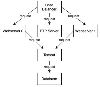
Example: IT system monitoring
The exemplary graph shown here represents the dependencies between the services of an IT infrastructure. For this purpose, server processes are modelled as graph nodes, with the processes linked by edges representing requests. The edges thus state that each node requires all its successors along the edges to function. It is also directly evident from the example that a graph database makes it possible to model the data model very close to the problem domain and thus make the data model intuitively understandable.
Graph databases and query languages
In the area of graph databases, in addition to offerings under purely commercial licences (e.g. TigerGraph, Amazon Neptune), there are also numerous with open source licences (e.g. Neo4j, ArrangoDB, OrientDB, JanusGraph), for some of which commercial licences are also offered. The most widespread graph database Neo4j, for example, is offered under a commercial as well as an open-source licence, although the use of the open-source variant is limited to a single server.
Another distinguishing feature is the query language used, with Cypher and Apache Tinkerpop Gremlin being the most important. While Cypher is mainly used by the graph database solution Neo4J, Gremlin emerged from the Apache Tinkerpop project and is supported by numerous graph databases such as Amazon Neptune or JanusGraph. Since the two languages are functionally equivalent and can be converted into each other automatically, knowledge of only one of the two languages is not a limiting factor in the choice of database system.
IT system monitoring: Gremlin queries
Basically, a distinction is made between local and global graph queries. While global queries include the entire graph, local queries are limited to a mostly small sub-area of the graph. Therefore, global queries are also runtime-critical for large graphs.
Local queries
A simple example of a local graph query in the graph above would be: To which server processes are the requests distributed by the load balancer?
The following query in Gremlin answers this question:
Gremlin queries follow the model of graph traversal. Starting from a set of nodes, which can also be pre-filtered by type or certain attribute values, the graph is traversed by following adjacent edges.
This part of the query states that the node with the attribute key name and the attribute value loadbalancer serves as the starting point for the traversal g:
This query is local, so the response time – if the starting node is known – does not depend on the size of the graph.
Global queries
The graph can also be used to assess how critical the failure of a component is for the overall system. For example, one can now formulate a query that indicates how many other processes require a process. To do this, all paths from the load balancer are taken into account. The corresponding Gremlin query is as follows:
This part of the query states that the set of all nodes serves as the starting point for the traversal g:
g.V()
Here, a map is created as a result, which contains the value of the attribute name as a key, which serves the readability of the result.
g.V().map(union(values('name'), ...)
Here, for each node, all incoming edges (_.in()) are iterated over until the node encountered has no more incoming edges (inE()). For each of these loops, the encountered nodes are counted (.emit().dedup().count()) after removing the duplicates and summarised in a list (.fold()):
This is an example of a global query that iterates over the entire graph, so its runtime depends on the size of the graph, unlike local queries.
Data modelling: mapping reality vs. query performance
For graph databases, data modelling has the advantage that the data model can be designed closely to reality and can be flexibly extended. On the other hand, the structure of the graph also has a direct influence on the efficiency of queries, as nodes can be reached more quickly via links. A good approach is therefore to start with the design of the data model close to reality and, in the case of performance problems with queries, to extend the graph accordingly with additional nodes and edges. This way, on the one hand, the representation of reality – and thus the understanding of the data model – is not impaired in its core, and on the other hand, new queries, for example, can be handled efficiently.
Performance and scale
Comparable to relational database systems, graph databases also offer options for indexing nodes or edges. This makes it possible to quickly access all nodes for which a set of attributes can be used as a key via an index. This result set can subsequently be used as a starting point for graph traversal. In addition to the indexing capabilities, the horizontal scalability of the graph database is a key criterion to avoid running into query performance problems as the amount of data continues to grow.
A licence-free solution for a scalable graph database is, for example, the open-source database Janusgraph, with which, among other things, a Hadoop cluster can be used as a storage backend. In addition, Apache Spark can be used as a graph compute engine to make the execution of global queries in graphs manageable up to the terabyte range.
RISC Software GmbH supports you at every stage of your process to generate the greatest possible value from your data. If you wish, this also includes the selection of the right tools for your needs – such as a graph database. Companies that do not yet have end-to-end data collection or do not yet use their data for such tasks have the opportunity to gradually increase the value they derive from their data. Building on its many years of expertise in the field of scalable NoSQL solutions, RISC Software GmbH can thus also serve as a reliable consulting and implementation partner for its customised solution in the field of NoSql systems and graph databases.